
Land and housing system outlook for South Australia 2026
Introduction
South Australia is currently experiencing strong rental and asset price increases alongside elevated levels of construction activity.
Across public discourse, these metrics are typically interpreted as indicators of rising prosperity and economic strength.
However, rapid price increases and elevated construction activity can also indicate the potential emergence of later phases of the long property cycle. This article explores whether recent trends in South Australia’s land and housing system are broadly consistent with the long-cycle framework. It also outlines three near-term scenarios for consideration.
The long-term cycle
The 18-year property cycle theory associated with author and economist Fred Harrison offers one framework for understanding the boom-and-bust dynamics of land, housing, and economic systems. Fred Harrison identified four key phases, which are summarised below.
The Recovery phase usually follows a major bust or downturn in the economy. His work suggests this phase lasts approximately seven years. The Recovery phase starts with heightened economic activity and higher-than-average housing construction. Towards the end of the phase, there may be a slight dip in economic activity as the recovery begins to moderate.
The second phase is the Explosive phase. His work suggests this phase can last approximately five years. The key characteristics of the Explosive phase are increased economic activity, increased speculation in land, rising rental and asset prices, increased development activity, and an overall perception of economic prosperity.
The third phase is the Winner’s Curse phase. His work suggests this is a short and intense phase that usually lasts approximately two years. During the Winner’s Curse phase, people take greater risks and speculate even more on assets, particularly land and housing, causing rents and asset prices to climb rapidly until further increases become unsustainable.
The fourth phase is the eventual Recession phase. His work suggests this phase can last three to five years. The Recession phase is characterised by an economic downturn and a significant pause in prices and construction activity.
Is the property cycle playing out now, particularly in South Australia?
According to cycle theory, the Recovery phase may have commenced around 2013 and concluded around 2019–2020. Activity in Australia, including South Australia, during this period appears broadly consistent with cycle theory.
The Recovery phase began with an economic recovery out of the post-GFC economic downturn and a significant increase in capital investment in the housing system between 2013 and 2017/18. This period was followed by a slight economic downturn in the years preceding the COVID-19 pandemic years, consistent with the mid-cycle dip at the end of the Recovery phase.
Cycle theory suggests the Explosive phase could have started around 2020. It appears activity in Australia, including in South Australia, was ready to increase in line with the theory timeframe.
Coincidentally, the economic conditions created by the pandemic response, particularly rising incomes, record levels of government grants, such as the HomeBuilder Grant, and very low interest rates accelerated and amplified this phase by bringing forward a significant volume of commitments by first home buyers and owner-occupiers that perhaps would otherwise have occurred over a longer period of time.
This significant increase in commitments, which drove the rise in asset prices in 2020 to early 2021, is evidenced by the increase in owner-occupier housing finance commitments as shown in Chart 1 below and the increase in asset prices in the same period as shown in Chart 2.
Chart 1: Owner-Occupiers Housing Finance Commitments
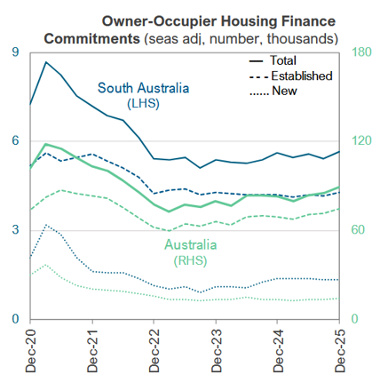
Australian Bureau of Statistics, Lending Indicators, December quarter 2025. Chart source: Department of Treasury and Finance SA
Chart 2: Asset Contract Prices - Houses
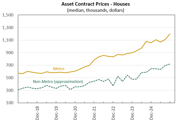
*Metro defined as the four South Australian Government Regions of Southern, Eastern, Northern, and Western
**Non Metro (approximation) = a combination of non-metro major towns, Adelaide Hills, and Gawler to best align with Consumer and Business Services rental price data.
Data source: Office of the Valuer General: Chart: B. Cooper
The drivers of asset price increases appear to broaden in 2021 and 2022. There was increasing economic activity and rising incomes, which arose from the post-COVID-19 lockdown economic boost, an unexpected population increase following the opening of borders, and a significant expansion in credit. These factors appeared to have helped two parallel and interconnected feedback loops unfold. One loop primarily involved landlords and tenants and the other primarily involved governments and first home buyers.
The first major feedback loop, which included landlords and tenants, appears to have occurred in the following way.
Rising prices fuelled a ‘we need more housing supply’ narrative.
The expanding narrative increased investor demand for land and housing.
Investors leveraged their rising equity and sought increased borrowing capacity.
Increased borrowing capacity expanded purchasing power and acquisitions.
Higher asset prices shifted required returns. Where rental conditions permitted, landlords adjusted rents toward prevailing market benchmarks.
Rental and asset price increases reinforced the narrative and attracted additional investors.
Chart 3 below shows the rapid increase in Investor Housing Finance Commitments from mid-2021 through to mid-2022. Chart 2 above shows the corresponding rapid increase in house prices across the same period.
Chart 3: Investor Housing Finance Commitments
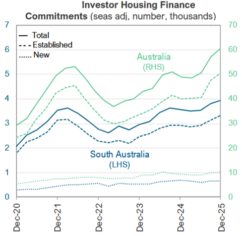
Australian Bureau of Statistics, Lending Indicators, December quarter 2025. Chart source: Department of Treasury and Finance SA
The second major feedback loop, which included first home buyers and governments, appears to have occurred in the following way.
A strong belief in the narrative, as well as concern that first home buyers might miss out, prompted governments to act.
Governments at national and state levels cut taxes and provided additional supports for first home buyers, including new housing programs that incorporated shared equity and government guarantees, which increased purchasing power.
Additional purchasing power enabled first home buyers to acquire land and housing at higher prices.
Asset price increases reinforced the narrative and encouraged additional responses from governments and lenders.
It does not appear that these loops operated independently from each other but rather reinforced each other through price signals that amplified demand for the same land and housing releases.
These intertwined loops set the stage for what may be the transition into the next phase of the cycle.
Have we entered the third phase?
According to cycle theory, we would have transitioned into the Winner’s Curse phase in 2024 or 2025. Based on a range of indicators, it is very possible that a transition into this phase of increased risk-taking and speculative behaviour may have already commenced or will commence soon. Indicators include:
Slowing rental price increases, primarily due to shrinking capacity for renting households to absorb continued contract rent increases, reduced landlords’ ability to continue increasing contract rents at the same rates. This is shown in Chart 4 below, where increases appear to slow in 2025.
Chart 4: Weekly Contract Rent – Houses.
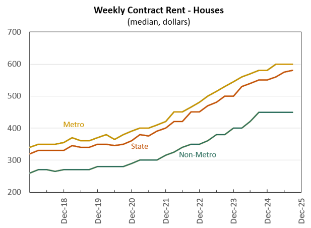
*Metro defined as the four South Australian Government Regions of Southern, Eastern, Northern, and Western.
**Non-metro defined as all other regions.
Data source: Consumer and Business Services. Chart B. Cooper
Gross Rental Yields (yields) for houses are falling from the long-term average. Using data from Consumer and Business Services and the Office of the Valuer General, we can suggest the yield has fallen from around an average of 3.2% to around 2.8% for metro Adelaide, as shown in Chart 5 below, noting yields for different house types and locations will be different, and not all yields will have followed the same pattern. SQM Research suggests the yield for houses in Adelaide has fallen from around 4 to around 3, noting SQM utilises a different data set to calculate their yield.
It’s important to note that yields have also reduced at the national level, but the fall is more pronounced in South Australia. This indicator builds upon the first indicator and suggests landlords may be increasingly reliant on future capital gains to justify investments.
Chart 5: Gross Rental Yield – Houses
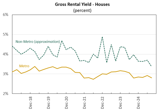
*Ratio using information from previous asset contract price and rental contract price data.
Data sources: Consumer and Business Services & Office of the Valuer General. Chart: B. Cooper.
Population growth is slowing and returning to the long-term average of around 1%, which may moderate overall underlying demand.
Slowing volume of residential land purchasers as shown in Chart 6 below, also suggests an upstream softening of demand, particularly for detached dwellings on the urban fringes, where a considerable proportion of additional houses have been constructed in recent years.
Chart 6: Residential Land Purchasers
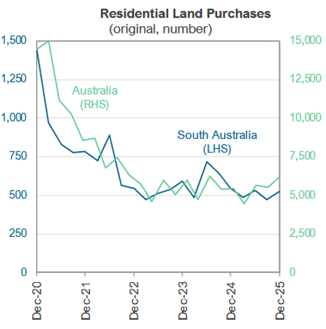
Australian Bureau of Statistics, Lending Indicators, December quarter 2025. Chart source: Department of Treasury and Finance SA
However, the two loops do not appear to be adjusting to these indicators. Rather, fears of missing out and increasing systemic risks appear to be the defining characteristics.
The first major feedback loop, which involves landlords and tenants, is now potentially unfolding in the following way.
The sustained ‘we need more housing supply’ narrative deepens the perception of persistent undersupply, attracting more investors (Chart 3).
Increased investor participation sustains strong demand for land and housing despite emerging risks.
Persistent demand reduces the usual moderating effects of rising interest rates and other constraints.
Continued demand places further upward pressure on asset prices (Chart 2) and supports elevated construction activity as shown in Charts 7 and 8 below.
Rising asset prices and construction activity validate the narrative, even as prices diverge from underlying income and yield fundamentals (Chart 5).
The second major feedback loop, which involves first home buyers and governments, is now potentially unfolding in the following way.
The sustained narrative deepens the perception of persistent undersupply and fears of first home buyers missing out.
In response, governments expand programs and financial supports and accelerate their release.
Expanded supports increase first home buyer purchasing power and borrowing capacity.
Higher borrowing levels increase leverage and sensitivities to interest rates and changing economic conditions.
Increased purchasing power contributes to further asset price growth.
Rising asset prices validate the housing shortage narrative and generate additional responses and risks for governments and lenders.
Chart 7: Dwelling Approvals per Month
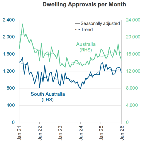
Australian Bureau of Statistics, Building Approvals, Australia, December 2025. Chart source: Department of Treasury and Finance SA
Chart 8: South Australian Dwelling Approvals and Commencements
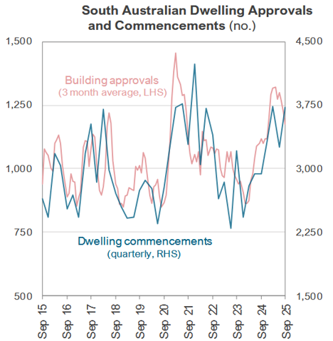
Australian Bureau of Statistics, Building Activity, Australia, September quarter 2025. Chart source: Department of Treasury and Finance SA
What is the outlook from here?
The land and housing system and broader economic systems are complex and interlinked. Outlining a definitive trajectory for the land and housing system using historical and current data alone with a strong level of confidence is extremely challenging.
The strength of cycle theory, and that economic and housing activity appears to be generally aligning with the theory in this cycle, means the overall theory can provide a reasonable framework to explore what could happen in the coming years with confidence. With reference to cycle theory, noting the theory is just one framework that can be utilised, three very broad-based scenarios have been prepared to help paint a picture of what could unfold in the coming years in the land and housing system.
Scenario 1: Current trajectory continues
In this scenario, the Winner’s Curse phase of the cycle does not occur in the way that it has unfolded in previous cycles, and the current trajectory of activity continues. Such a scenario could unfold as follows:
Asset prices continue to rise, enabling landlords to lift rents further.
Rental price growth accelerates beyond recent rates, intensifying cost-of-living pressures for tenants.
Expectations of continued price growth reinforce investor and first home buyer participation, increasing the volume of land purchases again.
Elevated demand sustains high levels of approvals and construction commencements, remaining above long-term averages and population growth.
In this scenario, the land and housing system would depart from the long-term property cycle and create an alternative cycle. There are issues with this scenario given that:
There is a point where renting households can no longer absorb continued rental price increases. This appears to be occurring now.
Household debt remains high, and there would be concerns around the extent that debt levels could continue to increase and concentrate at the rates they have occurred, particularly relative to incomes.
Scenario 2: Minor Downturn
In this scenario, there would be stagnation or a minor downturn in housing and housing-linked economic activity. This would be driven by a feedback loop that could unfold in many ways. Below is one illustrative pathway through which it could unfold.
Buyers and lenders reassess the sustainability of continued asset price growth.
As expectations weaken, demand for land and housing softens.
Weakening demand causes asset price increases to slow or stall.
In response to weaker price conditions, title owners delay releasing construction-ready sites.
Reduced volume of titles for sale slows new construction activity.
The contraction in construction generates ripple effects across employment, incomes, and broader economic activity.
As activity slows, lenders’ risk appetites tighten and households’ capacity and willingness to borrow contracts.
Tighter credit and reduced borrowing capacity further weaken demand for land and housing, reinforcing price weakness and validating the initial reassessment.
Scenario 3: Major Downturn
In this scenario, there could be a major downturn in housing and housing-linked economic activity that could come from within South Australia or Australia. It could also be caused by other events or downturns originating outside of Australia. The magnitude and duration would depend on the origin and severity of the disruption, but the feedback loops would be broader and more forceful than in a minor downturn. One illustrative pathway is as follows:
A significant disruption to economic stability materially weakens household and lender confidence.
As confidence deteriorates, demand for land and housing contracts sharply.
Reduced demand places sustained downward pressure on asset prices and transaction volumes.
In response to weakening prices and slower sales, landowners delay or withdraw construction-ready sites from the market.
Falling valuations and reduced turnover prompt lenders to tighten credit conditions and reassess risk exposures.
Tighter credit further constrains land purchases, development activity, and refinancing capacity.
Declining activity increases financial stress on builders and related businesses, reducing employment and household incomes.
As uncertainty deepens, households prioritise debt reduction and saving, weakening broader consumption and private investment.
Weaker economic activity and tighter credit further suppress housing demand, reinforcing pressure on asset prices and deepening the downturn.
Are there risks for South Australia?
There would be a myriad of challenges for Australia and South Australia should scenarios like two or three unfold. There would also be additional challenges for South Australia given:
Because investors, particularly from interstate, have been a significant driver of price growth in South Australia, they may have fewer ties to South Australia than South Australian owners, and may be more likely to sell in a downturn, which would amplify the downturn and its contractionary effects.
House construction currently represents a significant share of South Australia’s economy—more so than in most other states and territories. A downturn in housing construction could generate additional issues for South Australia’s economy.
Stamp duty revenue represents a significant share of the State Government’s budget, and a contraction in asset prices and/or transfers could amplify budgetary pressures, particularly at a time when government would be asked by industries and communities to stimulate the economy.
Conclusion
Cycle theory offers a strong framework to understand activity in the land and housing system, as well as the broader economy. This article highlights that activity in South Australia over the past 13 years appears broadly consistent with key characteristics of the first three phases of the long-term cycle. This suggests the theory also offers a reasonable framework to consider what could unfold in the coming years.
What is not foreseeable at this point is if or when there will be a transition into the end of the cycle, as well as the potential magnitude and severity of any downturn. All we can see, based on the work to date, is there is an emerging downturn risk. Further work is required to develop a better understanding of this risk, as well as how this could be mitigated as much as possible, and how we might respond to a downturn should one occur.
Changes to behaviour, regulation, and taxation would materially influence how the systems evolve going forward.
In our upcoming event, Housing: From the last four years to the next on 12 March 2026, these ideas will be explored further, as well as interventions governments could pursue to reduce the likelihood and impacts of a downturn.